本文为自己看别人写的tf代码时的总结,希望以后会用到.第一部分主要是关于conv layer和变量定义还有BN trick的相关总结,主要以代码为主
一些要提前注意的点
- 一个好的习惯是将一些常用的tf中已经有的函数重新封装一遍,这种封装主要体现在变量定义和操作定义上面.其好处在于将函数的参数变少
- 对于一些常用的conv和deconv操作,一定要弄清楚NHWC的参数值,避免出错
- 定义变量一定要有
name
- tf的数据格式是NHWC
变量定义
直接利用tf定义
1 2 3
| import tensorflow as tf weights = tf.truncated_normal(name, shape, stddev) biases = tf.constant(0.0, shape)
|
封装版1.0
1 2 3 4 5 6 7 8 9
| import tensorflow as tf def weight_variable(shape, stddev=0.02, name=None): initial = tf.truncated_normal(shape, stddev=stddev) return tf.Variable(initial) if name is None else tf.get_variable(name, initializer=initial) def bias_variable(shape, name=None): initial = tf.constant(0.0, shape) return tf.Variable(initial) if name is None else tf.get_variable(name, initializer=initial) weights = weight_variable(name, shape) biases = bias_variable(name, shape)
|
这里要注意的就是在有无name的情况下选择的初始化函数.
封装版2.0
1 2 3 4 5 6 7 8 9 10 11 12 13 14 15 16 17 18 19 20 21 22 23 24 25 26 27 28 29 30 31 32 33 34
| import tensorflow as tf def _variable_on_cpu(name, shape, initializer): """Helper to create a Variable stored on CPU memory. Args: name: name of the variable shape: list of ints initializer: initializer for Variable Returns: Variable Tensor """ with tf.device('/cpu:0'): var = tf.get_variable(name, shape, initializer=initializer) return var def _variable_with_weight_decay(name, shape, stddev, wd): """Helper to create an initialized Variable with weight decay. Note that the Variable is initialized with a truncated normal distribution. A weight decay is added only if one is specified. Args: name: name of the variable shape: list of ints stddev: standard deviation of a truncated Gaussian wd: add L2Loss weight decay multiplied by this float. If None, weight decay is not added for this Variable. Returns: Variable Tensor """ var = _variable_on_cpu(name, shape, tf.truncated_normal_initializer(stddev=stddev)) if wd: weight_decay = tf.mul(tf.nn.l2_loss(var), wd, name='weight_loss') tf.add_to_collection('losses', weight_decay) return var weights = _variable_with_weight_decay('weights', shape=[5, 5, 64, 64],stddev=1e-4, wd=0.0) biases = _variable_on_cpu('biases', [64],tf.constant_initializer(0.1))
|
构建一个conv layer
tf中的conv2d
1
| tf.nn.conv2d(input, filter, strides, padding, use_cudnn_on_gpu=True, data_format=None, name=None)
|
按照官网的API,有以下几点需要注意:
- 这里的
input和filter的tensor_shape要求一致,
input的shape为:[batch, in_height, in_width, in_channels]filters的shape为:[filter_height, filter_width, in_channels, out_channels]- 默认数据格式
data_format是"NHWC"
padding一般取"SAME",即保持卷积之后的尺寸不变strides的shape为:[batch_skip, stride_h_skip, stride_w_skip, in_channels_skip],由于batch里面的每一个训练数据和输入的每个通道都会被用于训练,因此官方要求strides的使用格式应该是[1, stride_skip, stride_skip, 1].第二个和第三个代表窗口(卷积核)的滑动步长,一般是一样的.
掌握这个函数的用法之后就会发现,定义一层普通的conv layer只需要分三步:
- 定义好
weights,biases,strides`
- 应用函数
tf.nn.conv2d(input, weights, strides, name),tf.nn.bias_add(conv, biases)
- 选择进行其他操作,如使用激活函数/池化/正则化
注意,由于整个网络的输入不一定是规则的(比如GAN,输入的是一个1-D的noise),所以这个时候一般采用tf.matmul(input, W) + b和tf.reshape方式构建第一个conv layer,进而将输入转化成为标准的tensor
进一步地,利用上面的变量定义封装2.0,可以构建一个conv->pool->norm:
1 2 3 4 5 6 7 8 9 10
| import tensorflow as tf with tf.variable_scope('conv') as scope: weights = _variable_with_weight_decay('weights', shape=[5, 5, 3, 64], stddev=1e-4, wd=0.0) conv = tf.nn.conv2d(images, kernel, [1, 1, 1, 1], padding='SAME') biases = _variable_on_cpu('biases', [64], tf.constant_initializer(0.0)) bias = tf.nn.bias_add(conv, biases) conv = tf.nn.relu(bias, name=scope.name) _activation_summary(conv1) pool = tf.nn.max_pool(conv1, ksize=[1, 3, 3, 1], strides=[1, 2, 2, 1], padding='SAME', name='pool') norm = tf.nn.lrn(pool1, 4, bias=1.0, alpha=0.001 / 9.0, beta=0.75, name='norm')
|
变量初始化的Tricks
对于神经网络的训练过程而言,梯度消失是一个很重的问题,而实践证明,weights的初始化对于梯度的影响很大.所以从几个不同的方面有几种不同的解决办法可以借鉴一下
基于方差方面的考量,我们认为为了使得网络中信息更好的流动,每一层输出的方差应该尽量相等,于是xavier_init方法应运而生,这种方法在2010年被提出,近几年才得到关注,见paper Understanding the Difficult of Training Deep Feedforward Neural Networks
其思路很简单,把weights的方差固定为2/(n_in+n_out),其中n_in和n_out是filters的shape[2]和shape[3],具体见下面的代码
1 2 3
| def weight_variable_xavier_initialized(shape, constant=1, name=None): stddev = constant * np.sqrt(2.0 / (shape[2] + shape[3])) return weight_variable(shape, stddev, name=name)
|
直接使用Batch Normalization Layer.我们想要的是在非线性activation之前,输出值应该有比较好的分布(例如高斯分布)以便于back propagation时计算gradient,更新weights,Batch Normalization将输出值强行做一次Gaussian Normalization和线性变换:
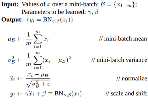
Batch Normalization中所有的操作都是平滑可导,这使得back propagation可以有效运行并学到相应的参数γ,β.需要注意的一点是Batch Normalization在training和testing时行为有所差别.Training时μβ和σβ由当前batch计算得出;在Testing时μβ和σβ应使用Training时保存的均值或类似的经过处理的值,而不是由当前batch计算.
使用BN的方法可以自己实现,也可以直接使用tf的contrib模块里面的现成函数.
1 2 3 4 5 6 7 8 9 10 11 12 13 14 15 16 17 18 19 20
| import tensorflow as tf def batch_norm(x, nb_filters_out, phase_train, scope='bn', decay=0.9, eps=1e-5, stddev=0.02): with tf.variable(scope): beta = tf.get_variable(name='beta', shape=[nb_filters_out], initializer=tf.constant_initializer(0.0), trainable=True) gamma = tf.get_variable(name='gamma', shape=[nb_filters_out], initializer=tf.random_normal_initializer(1.0, stddev), trainable=True) batch_mean, batch_var = tf.nn.moments(x, [0, 1, 2], name='moments') ema = tf.trian.ExponentialMovingAverage(decay=decay) def mean_var_with_update(): ema_apply_op = ema.apply([batch_mean, batch_var]) with tf.control_dependencies([ema_apply_op]): return tf.identity(batch_mean), tf.identity(batch_var) mean, var = tf.cond(phase_train, mean_var_with_update, lambda: (ema.average(batch_mean), ema.average(batch_var))) normed = tf.nn.batch_normalization(x, mean, var, beta, gamma, eps) tf.contrib.layers.batch_norm(x, decay=0.9, center=True, scale=True, epsilon=1e-5, is_training=True, scope='bn')
|